Input files

Preparing the datafiles

To use edxia, we assume that you have a multispectral BSE/EDS maps (i.e. an hyperspectral maps that has been generated qualitatively or quantitatively). The data must be exported from the microscopy software to be made available to edxia.

edxia requires raw maps in text format (csv-type) from the microscope/EDS software. The text format is required to easily accept data from various acquisition software. If needed scikit-image <https://scikit-image.org/>_ or `imageJ can be used to batch convert images into corresponding text format.

Note

At the moment, edxia is localization unaware and uses “.” as the decimal separator (per the default of numpy internals). However, the field separator and normalization (min and max values allowed) can be configured.

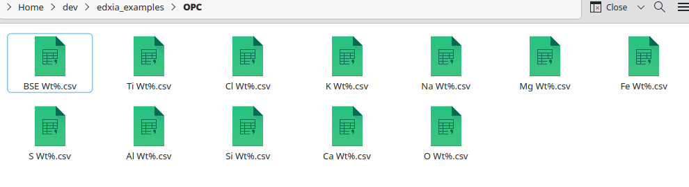
All maps from a a set must be in the same folder. Using the default classes, the user only select the BSE map, and the program find the other maps available based on the filenames, by replacing BSE with a known set of chemical symbols for the elements. For example, the maps in the edxia article [1] follow the pattern <element> Wt%.txt; where <element> is either BSE or one of Ca, Si, S, Al, Fe, …

The list of allowed elements are currently defined in edxia.utils.chemistry.elements.

Warning

It is common to acquire the BSE at a higher resolution than the EDS. edxia requires that the resolution are the same for BSE and EDS maps. If it is not the case, the BSE map can be downsized using imageJ, or in the glue interface plugins::edxia:BSE editor.

The method to export the data from the microscopy software (e.g. Aztec from Oxford Instruments, or Esprit from Bruker) is not described in this documentation. Please refer to your manual as it vary from software to software and version to version.

To get familiar with the software, and follow the doc step-by-step, the data can be dowloaded from the Zenodo repository. The dataset contains the main maps used in the edxia article [1]. More details on their acquisition parameters and quantification process can be found in the corresponding article.

In the Qt Glue interface

Import

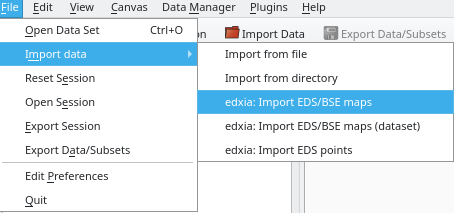
To open a new dataset through the glue interface, use the file::import data::edxia: Import EDS/BSE maps.

The wizard to import EDS/BSE multispectral maps into the glueviz interface opens up. The forms at the top of the window and in the second tab Format can be used to load the maps.

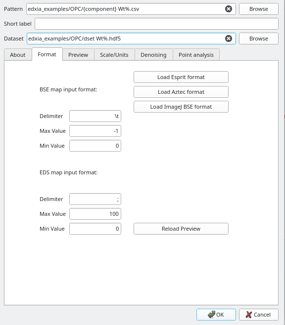
The first step is to indicate the pattern that will be used to load the maps. It can be entered manually, or alternatively, the user can select the BSE map to generate the pattern. Using the top browse button, the user can find the BSE to load, and edxia will generate the pattern.

The short label field can be filled to customize the name of the maps in the interface. A name is automatically created from the pattern.

The third field dataset is used to saved the transformed data produced by edxia. It can be used to easily reupload the data into glue. If left empty, the dataset will not be created.

The bottom part (the Format tab) contains the directives to load the data, one for the BSE map, and one for the EDS maps. The separator for the CSV-type files (e.g. ‘,’, ‘t’ or ‘ ‘) can be provided as well as the min and max values allowed in the datafile. These values are used to normalize the data. This is especially important for EDS maps which are on a absolute scale. A value of ‘-1’ indicates that the maximum value in the file will be used for the normalization.

For convenience, the typical formats from known pieces of software can be easily loaded with the buttons on the right of the window.

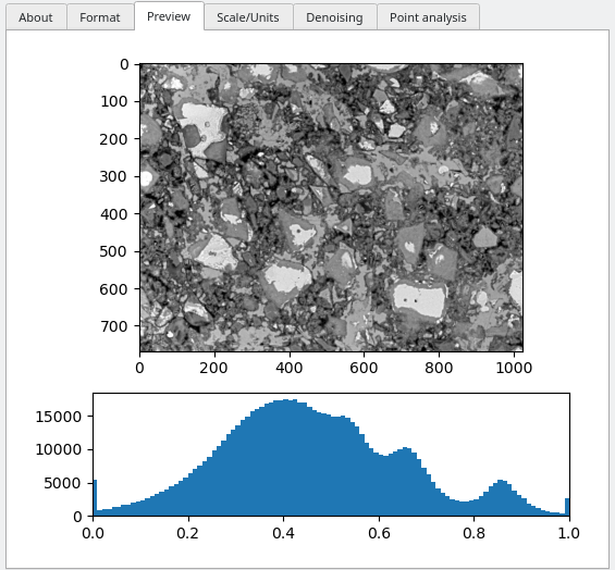
The reload preview allows to test the format by displaying the BSE on the next tab, with its histogram. Here is an example of a successful loading of the BSE:

The next tabs concern the normalization of the maps and the parameters for the edxia algorithms.

Scale/units

The tab scale/units is used to provide further information about the maps.

The first option Pixel size is the length of pixel in nanometer. This value is optional and can be obtained from the microscopy software. It is used for display only; if it is provided the maps plots in glue will be displayed in micron. If not provided (i.e. if the value is 0), the maps will be shown in pixels

The input units choice needs to be set up according to the normalization applied to the EDS map by the microscopy software. The three choices are % Atomic, % Weight and Weight. The first two options are normalized so that the sum of the component concentrations is 100 %. The last two options are to be used when an EDS map represents the concentration of an element expressed in mass (e.g. g/100g). The atomic unit are the stoichiometric concentrations.

The output units are options for edxia to change the input units on-the-fly. If the Normalize option is chosen, the sum of the detected elemental concentrations will be 100 %. If the % Atomic (default option) is selected, EDS maps in % Weight and Weight will be transformed into % Atomic.

The Compute sum of oxide is only available if the input units is set as Weight. If selected the sum of oxide (the sum of the oxides (CaO, SiO2, Al2O3, …) mass) will be computed. This calculation takes place before the atomic conversion if any.

Denoising

In the Denoising tab, the denoising algorithm to be used for the EDS map can be selected. The BSE map is not denoised by the edxia algorithm as it assumed to be of higher quality. More information on denoising can be found in the original publication (open-access).

The different options available are:

No Filter

No denoising algorithm is applied, not recommended for practical applications

Total Variation

The total variation algorithm from A. Chambolle, as implemented by Scikit-image. This is the recommended option as it is generally a robust and reliable option. The parameter of “0.1” is generally a good choice.

Mean filter

The standard uniform filter as implemented in [scipy](https://docs.scipy.org/doc/scipy/reference/generated/scipy.ndimage.uniform_filter.html#scipy.ndimage.uniform_filter). Typically not recommended as it will blur edges

Median filter

The median filter as implemented in [scipy](https://docs.scipy.org/doc/scipy/reference/generated/scipy.ndimage.median_filter.html#scipy.ndimage.median_filter). Typically not recommended as it will blur edges.

Median filter

The gaussian filter as implemented in [scipy](https://docs.scipy.org/doc/scipy/reference/generated/scipy.ndimage.gaussian_filter.html#scipy.ndimage.gaussian_filter). Typically not recommended as it will blur edges.

Joint bilateral filter

A joint bilateral filter as implemented in OpenCV. OpenCV is an optional library. If cv2.ximgproc is not installed (from the opencv-contrib-python package), this option will not be available. This option can lead to the best result as it uses a edge-preserving algorithm, using the high-resolution BSE map to define the edges (ref1, ref2). This is not a robust algorithm and the parameters need to be carefully adjusted to the specific maps. The parameter Sigma S corresponds to the Sigma Color parameter of the opencv documentation; it is the gaussian filter sigma in the EDS concentration space. The parameter Sigma R corresponds to the Sigma Space parameter of the opencv documentation; it is the filter sigma which defines how far two pixels can influence each other in the filter.

Segmentation filter

This is a “homemade” filter. It first defines a SLIC segmentation for the BSE map using the parameters Nb regions and Compactness. Then a mean filter is used inside each region to set a singular value per region. In its current form, this filter was not found to be very reliable.

Point analysis

To come !

In the Python API

Warning

In construction

The text format must be one of the various csv-type formats. The exact delimiter, and normalization to apply are described by edxia.io.raw_io.TextMapFormat. Several predefined format are available in this module (edxia.io.raw_io).

This is the default in :mod:edxia: but the user can defines it’s own loading functions by specializing edxia.io.loader.base_loader.AbstractLoader.